In the spring of 2018, I worked on an encoding and decoding project for a course about machine learning in Python. I studied the ways neuroscientific data can be analyzed to form predictions of how humans perceive the world. For this set of data, we rely on voxels (the unit of array elements in neuroimaging) and can measure various characteristics from them such as intensity, size, and shape. With these sorts of issues, supervised learning can be used to decode images to relate brain images to behavioral or clinical observations. The predictions made by these supervised forms of learning can then be cross-validated to assess how those results from these individual experiments can be generalized to broader patterns in neuroscience data. We’ll be using a Python module called nilearn for this analysis.
In this post, I’d like to explain how to apply different statistical methods to real data in the field of neuroscience. Biophysical models can be made to estimate empirical evidence brought by the biology and neuroscience, and using descriptions of neurons (complete with dendrites, synapses, and axons). These mathematical frameworks are common throughout various problems in genetics and embryology, but I’d like to focus on their role in neuron models. Through various methods such as sodium and potassium ion channels (which activate through spiking at threshold potentials), we can uncover predictive models based on the causality of this data.
We can test the performance of these, and other, models by using them as predictive models of encoding. Given a stimulus, will the model be able to predict the neuronal response? Will it be able to predict spike times (the potential received by a neuron) observed in real neurons when driven by the same stimulus – or only the mean firing rate or PSTH (Peristimulus time histogram)? Will the model be able to account for the variability observed in neuronal data across repetitions?
A sequence, or “train”, of spikes may contain information based on different coding schemes. In motor neurons, for example, the strength at which an innervated muscle is contracted depends solely on the “firing rate”, the average number of spikes per unit time (a “rate code”). At the other end, a complex ‘temporal code’ is based on the precise timing of single spikes. They may be locked to an external stimulus such as in the visual and auditory system or be generated intrinsically by the neural circuitry.
Testing the performance of models addresses yet a bigger question. What information is discarded in the neural code? What features of the stimulus are most important? If we understand the neural code, will we be able to reconstruct the image that the eye is actually seeing at any given moment from spike trains observed in the brain? The problem of decoding neuronal activity is central both for our basic understanding of neural information processing and for engineering ‘neural prosthetic’ devices that can interact with the brain directly. Given a spike train observed in the brain, can we read out intentions, thoughts, or movement plans? Can we use the data to control a prosthetic device?
While neural codes are characterized in terms of these encoding views (i.e., how the neurons map the stimulus onto the features of spike responses), these are often investigated and validated using decoding. From the decoding viewpoint, rate coding is operationally defined by counting the number of spikes over a period of time, without taking into account any correlation structure among spikes. Any scheme based on such an operation is equivalent to decoding under the stationary Poisson assumption, because the number of spikes over a period of time, or the sample mean of interspike intervals (ISIs), is a sufficient statistic for the rate parameter of a homogeneous Poisson process.
Since neuronal response is stochastic, a one-to-one mapping of stimuli into neural responses does not exist, causing a mismatch between the two viewpoints of neural coding. For a model to be stochastic, it must operate like a function randomly determined. We can create generalized linear models (GLMs) that have been used for mathematical analysis of neuronal data which have been shown to correspond with models used specifically in neuroscience. These similarities occur when the spiking history term contains only the last spike and a log-link function is used (e.g., soft-threshold integrate-and-fire models (Paninski et al., 2008)).
Due to its complex and indirect acquisition process, neuroimaging data often have a low signal-to-noise ratio. They contain trends and artifacts that must be removed to ensure maximum machine learning algorithms efficiency. Signal cleaning includes: detrending removes a linear trend over the time series of each voxel. This is a useful step when studying fMRI data, as the voxel intensity itself has no meaning and we want to study its variation and correlation with other voxels. Detrending can be done thanks to SciPy (scipy.signal.detrend).
Normalization consists in setting the time series variance to 1. This harmonization is necessary as some machine learning algorithms are sensible to different value ranges. Frequency filtering consists in removing high or low frequency signals. Low-frequency signals in fMRI data are caused by physiological mechanisms or scanner drifts. Filtering can be done thanks to a Fourier transform (scipy.fftpack.fft) or a Butterworth filter (scipy.signal.butter).
In this project, I reconstructed visual images by combining local image bases of multiple scales, whose contrasts were independently decoded from fMRI activity by automatically selecting relevant voxels and exploiting their correlated patterns. Binary-contrast, 10 × 10-patch images (2^100 possible states) were accurately reconstructed without any image prior on a single trial or volume basis by measuring brain activity only for several hundred random images. Reconstruction was also used to identify the presented image among millions of candidates. The results suggest that our approach provides an effective means to read out complex perceptual states from brain activity while discovering information representation in multivoxel patterns.
Neuroimaging data often come as Nifti files, 4-dimensional data (3D scans with time series at each location or voxel) along with a transformation matrix (called affine) used to compute voxel locations from array indices to world coordinates. The tools we use convert the images from 4-dimensional images to 2-dimensional arrays. Masking Neuroimaging data are represented in 4 dimensions: 3 spatial dimensions, and one dimension to index time or trials. Scikit-learn algorithms, on the other hand, only accept 2-dimensional samples × features matrices. Depending on the setting, voxels and time series can be considered as features or samples. For example, in spatial independent component analysis (ICA), voxels are samples. The reduction process from 4D-images to feature vectors comes with the loss of spatial structure. It however allows to discard uninformative voxels, such as the ones outside of the brain. Such voxels that only carry noise and scanner artifacts would reduce SNR and affect the quality of the estimation. The selected voxels form a brain mask. Such a mask is often given along with the datasets or can be computed with software tools such as FSL or SPM.
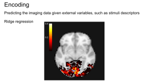
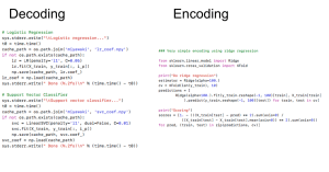
In the experiment of Miyawaki et al. (2008) several series of 10×10 binary images are presented to two subjects while activity on the visual cortex is recorded. The visual reconstruction steps are shown to the left. In the original paper, the training set is composed of random images (where black and white pixels are balanced) while the testing set is composed of structured images containing geometric shapes (square, cross…) and letters. Here, for the sake of simplicity, we consider only the training set and use cross-validation to obtain scores on unseen data. In the following example, we study the relation between stimuli pixels and brain voxels in both directions: the reconstruction of the visual stimuli from fMRI, which is a decoding task, and the prediction of fMRI data from descriptors of the visual stimuli, which is an encoding task.
Sources
Abraham et al. (2014). “Machine learning for neuroimaging with scikit-learn” Frontiers in Neuroinformatics.
Miyawaki et. al. (2004). “Visual Image Reconstruction from Human Brain Activity using a Combination of Multiscale Local Image Decoders” Neuron.
Paninski, L., Brown, E. N., Iyengar, S., & Kass, R. E. (2008). Statistical analysis of neuronal data via integrate-and-fire models. Chapter in Stochastic Methods in Neuroscience, eds. Laing, C. & Lord, G. Oxford: Oxford University Press.


